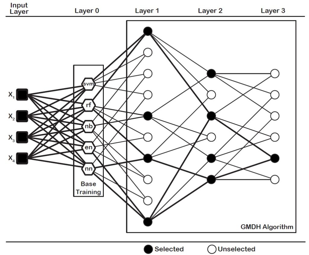
The dce-GMDH type neural network algorithm is a heuristic self-organizing algorithm to assemble the well-known classifiers. Find out how to apply dce-GMDH algorithm for binary classification in R.
In this tutorial, we will work dce-GMDH type neural network approach for binary classification. Before we start, we need to divide data into three parts; train, validation and test sets. We use train set for model building. We utilize validation set for neuron selection. Last, we show the performance of the model on test set.
Check Out: Feature Selection and Classification via GMDH Algorithm in R
In this tutorial, we will implement the algorithm on urine dataset, also used in the work done by Dag et al. (2022), available in boot package (Canty and Ripley, 2020). Before we go ahead, we load dataset and start to process the data.
data(urine, package = "boot")
After loading dataset, let’s exclude missing values to work on the complete dataset.
data <- na.exclude(urine)
head(data)
##   r gravity   ph osmo cond urea calc
## 2 0   1.017 5.74  577 20.0  296 4.49
## 3 0   1.008 7.20  321 14.9  101 2.36
## 4 0   1.011 5.51  408 12.6  224 2.15
## 5 0   1.005 6.52  187  7.5   91 1.16
## 6 0   1.020 5.27  668 25.3  252 3.34
## 7 0   1.012 5.62  461 17.4  195 1.40
Also Check: How to Handle Missing Values in R
We need to define the output variable as factor and input variables as matrix.
x <- data.matrix(data[,2:7])
y <- as.factor(data[,1])
We need to divide data into three sets; train (60%), validation (20%) and test (20%) sets. Then, we obtain the number of observations in each fold.
nobs <- dim(data)[1]
ntrain <- round(nobs*0.6,0)
nvalid <- round(nobs*0.2,0)
ntest <- nobs-(ntrain+nvalid)
Now let’s obtain the indices of train, validation and test sets. Before we obtain the indices, we shuffle the indices to prevent any bias based on order. For reproducibility of results, let’s fix the seed number to 1234.
set.seed(1234)
indices <- sample(1:nobs)

train.indices <- sort(indices[1:ntrain])
valid.indices <- sort(indices[(ntrain+1):(ntrain+nvalid)])
test.indices <- sort(indices[(ntrain+nvalid+1):nobs])
We can construct train, validatation and test sets.
x.train <- x[train.indices,]
y.train <- y[train.indices]
x.valid <- x[valid.indices,]
y.valid <- y[valid.indices]
x.test <- x[test.indices,]
y.test <- y[test.indices]
After obtaining train, validation and test sets, we can use dce-GMDH type neural network algorithm. dce-GMDH algorithm is available in GMDH2 package (Dag et al., 2019).
library(GMDH2)
model <- dceGMDH(x.train, y.train, x.valid, y.valid, alpha = 0.6, maxlayers = 10, maxneurons = 15, exCriterion ="MSE", verbose = TRUE)

##  Structure :
##
##  Layer     Neurons     Selected neurons               Min MSE
##      0           5                    5     0.141036573711885
##      1          10                    1     0.139424256676092
##
##  External criterion   : Mean Square Error
##
##  Classifiers ensemble : 2 out of 5 classifiers are assembled.
##
##  naiveBayes
##   cv.glmnet
Also Check: How to Clean Data in R
Now, let’s obtain performance measures on test set.
y.test_pred <- predict(model, x.test, type = "class")
confMat(y.test_pred, y.test, positive = "1")

## Confusion Matrix and Statistics
##
##     reference
## data 1 0
##    1 4 2
##    0 2 8
##
##
##      Accuracy             :   0.75
##      No Information Rate  :   0.625
##      Kappa                :   0.4667
##      Matthews Corr Coef   :   0.4667
##      Sensitivity          :   0.6667
##      Specificity          :   0.8
##      Positive Pred Value  :   0.6667
##      Negative Pred Value  :   0.8
##      Prevalence           :   0.375
##      Balanced Accuracy    :   0.7333
##      Youden Index         :   0.4667
##      Detection Rate       :   0.25
##      Detection Prevalence :   0.375
##      Precision            :   0.6667
##      Recall               :   0.6667
##      F1                   :   0.6667
##
##      Positive Class       :   1
In this model, dce-GMDH algorithm assembles the classification algorithms, naive bayes and elastic net logistic regression, contributing the classification performance. This ensemble algorithm classified 75.0% of individuals in a correct class. Also, sensitivity and specificity are calculated as 0.6667 and 0.8, respectively.
The application of the codes is available in our youtube channel below.
Don’t forget to check: 6 Ways of Subsetting Data in R
References
Dag, O., Karabulut, E., Alpar, R. (2019). GMDH2: Binary Classification via GMDH-Type Neural Network Algorithms – R Package and Web-Based Tool. International Journal of Computational Intelligence Systems, 12:2, 649-660.
Dag, O., Kasikci, M., Karabulut, E., Alpar, R. (2022). Diverse Classifiers Ensemble Based on GMDH-Type Neural Network Algorithm for Binary Classification. Communications in Statistics – Simulation and Computation, 51:5, 2440-2456.
Canty, A., Ripley, B. (2020). boot: Bootstrap R (S-Plus) Functions. R package version 1.3-25.

Leave a Reply