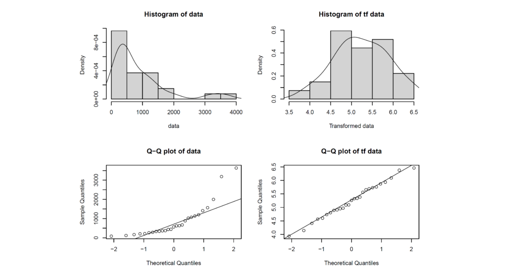
Box-Cox transformation is commonly used remedy when the normality is not met. This comherensive guide includes estimation techniques and use of Box-Cox transformation in practice. Find out how to apply Box-Cox transformation in R.
In this tutorial, we will work on Box-Cox transformation in R. Firstly, we will mention two types of estimation techniques for Box-Cox transformation parameter. These are maximum likelihood estimation (MLE) and estimation via normality tests. Secondly, we will work how to apply Box-Cox transformation in practice. Then, we will implement Box-Cox transformation in R. Last, we will find mean and confidence interval after conducting Box-Cox transformation in R.
In this part, we will use textile dataset available in AID package (Asar et al., 2017).
library(AID)
data(textile)
data <- textile[,1]
Check Out: How to Assess Normality in R
1. Estimation Techniques for Box-Cox Transformation Parameter
In this part, we include two types of estimation for Box-Cox transformation parameter. These techniques use likelihood and normality tests.
1.1. Estimating Box-Cox Transformation Parameter via MLE
We include maximum likelihood estimation of Box-Cox power transformation parameter. There are three ways of this estimation. Firstly, there exist boxcoxnc() function available AID package (Asar et al., 2017). Secondly, we use boxcox() function available in MASS package (Venables and Ripley, 2002). Last, we apply powerTransform function available in car package (Fox and Weisberg, 2019).
library(AID)
out <- boxcoxnc(data, method = "mle", lambda = seq(-2,2,0.0001), verbose = F, plot = F)
out$lambda.hat
## [1] -0.0474

library(MASS)
out <- boxcox(data~1, lambda = seq(-2,2,0.0001), plotit = F)
out$x[which.max(out$y)]
## [1] -0.0474

library(car)
out <- powerTransform(data, family = "bcPower")
out$lambda
##        data
## -0.04740941
1.2. Estimating Box-Cox Transformation Parameter via Normality Tests
In this part, we include the estimation of Box-Cox transformation parameter via normality tests. Asar et al. (2017) included Shapiro–Wilk, Anderson–Darling, Cramer-von Mises, Pearson Chi-square, Shapiro-Francia, Lilliefors and Jarque–Bera tests for the estimation of Box-Cox power transformation parameter. They compared estimation performance of the normality tests via Monte Carlo simulation study. Shapiro-Wilk test performs better for the estimation of Box-Cox power transformation parameter compared to others. On the other hand, Pearson chi-square test is the worst performing method for estimating Box-Cox transformation parameter.
library(AID)
out <- boxcoxnc(data, method = "sw", lambda = seq(-2,2,0.0001), verbose = F, plot = F)
out$lambda.hat
## [1] -0.0605

out <- boxcoxnc(data, method = "ad", lambda = seq(-2,2,0.0001), verbose = F, plot = F)
out$lambda.hat
## [1] -0.0772

out <- boxcoxnc(data, method = "cvm", lambda = seq(-2,2,0.0001), verbose = F, plot = F)
out$lambda.hat
## [1] -0.1014

out <- boxcoxnc(data, method = "sf", lambda = seq(-2,2,0.0001), verbose = F, plot = F)
out$lambda.hat
## [1] -0.0561

out <- boxcoxnc(data, method = "lt", lambda = seq(-2,2,0.0001), verbose = F, plot = F)
out$lambda.hat
## [1] -0.0562

out <- boxcoxnc(data, method = "jb", lambda = seq(-2,2,0.0001), verbose = F, plot = F)
out$lambda.hat
## [1] -0.065

out <- boxcoxnc(data, method = "pt", lambda = seq(-2,2,0.0001), verbose = F, plot = F)
out$lambda.hat
## [1] 0.0138
Also Check: Shapiro-Wilk Test for Univariate and Multivariate Normality in R
2. How to Apply Box-Cox Transformation in Practice
In this part, we work on implementing Box-Cox transformation and how to find mean and confidence interval after conducting Box-Cox transformation in R.
2.1. Implementing Box-Cox Transformation in R
We use Shapiro-Wilk test statistic to estimate Box-Cox transformation parameter.

After power transformation parameter is obtained, we can assess the normality of transformed data via Shapiro-Wilk test.
library(AID)
out <- boxcoxnc(data, method = "sw", lambda = seq(-2,2,0.0001))
##   Box-Cox power transformation
## -------------------------------------------------------------------
##   data : data
##
##   lambda.hat : -0.0605
##
##
##   Shapiro-Wilk normality test for transformed data (alpha = 0.05)
## -------------------------------------------------------------------
##
##   statistic  : 0.9877619
##   p.value    : 0.9821313
##
##   Result     : Transformed data are normal.
## -------------------------------------------------------------------

out$lambda.hat
## [1] -0.0605

out$tf.data
##  [1] 5.383140 4.971305 4.804571 4.907881 4.738234 4.568397 4.414510 4.143933 3.939296
## [10] 5.871742 5.764323 5.341807 5.660345 5.326684 5.088678 5.094968 4.895282 4.602013
## [19] 6.463622 6.382461 6.092968 5.938188 5.690482 5.264755 5.731956 5.564541 4.952131
2.2. How to Find Mean and Confidence Interval After Conducting Box-Cox Transformation in R
We apply Box-Cox transformation and find transformation parameter (-0.0605). Then, we can find mean and confidence interval for back transformed data with confInt() function available in AID package.
library(AID)
out <- boxcoxnc(data, method = "sw", lambda = seq(-2,2,0.0001), verbose = F, plot = F)

confInt(out, level = 0.95)
##   Back transformed data
## ---------------------------------------------
##          Mean     2.5%    97.5%
## data 549.3418 379.9816 800.8924
## ---------------------------------------------

confInt(out, level = 0.99)
##   Back transformed data
## ---------------------------------------------
##          Mean     0.5%    99.5%
## data 549.3418 334.4112 916.3863
## ---------------------------------------------
Also Check: How to Clean Data in R
The application of the codes is available in our youtube channel below.
Don’t forget to check: 6 Ways of Subsetting Data in R
References
Asar, O., Ilk, O., Dag, O. (2017). Estimating Box-Cox Power Transformation Parameter Via Goodness-of-Fit Tests. Communications in Statistics – Simulation and Computation, 46:1, 91-105.
Fox, J., Weisberg, S. (2019). An R Companion to Applied Regression, Third Edition. Thousand Oaks CA: Sage.
Venables, W.N., Ripley, B.D. (2002). Modern Applied Statistics with S. Fourth Edition. Springer, New York.

0 Comments
2 Pingbacks