Variance homogeneity is a severe assumption for ANOVA. This inclusive guide includes heteroscedastic ANOVA tests for one-way independent designs in R. Find out how to apply heteroscedastic ANOVA tests in R.
In this tutorial, we will work on five heteroscedastic ANOVA tests for one-way designs tests in R.
- Alexander-Govern test
- Brown-Forsythe test
- James second order test
- Welch’s heteroscedastic F test
- Welch’s heteroscedastic F test with trimmed means and Winsorized variances
These five heteroscedastic tests are compared via Monte Carlo simulation study in the work done by Dag et al. (2018). Alexander-Govern, James second order and Welch’s heteroscedastic F tests are recommended for use when the variance homogeneity assumption is not met.
Alexander-Govern, Brown-Forsythe, James second order, Welch’s heteroscedastic F tests test the null hypothesis of the equality of means. Welch’s heteroscedastic F test with trimmed means and Winsorized variances tests the equality of trimmed means.
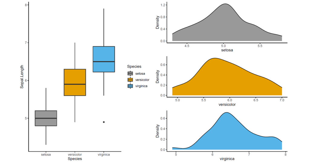
In this part, we will use iris data set available in R. We will use sepal length as a response variable and species as a grouping variable. Before we go ahead, let’s obtain descriptive statistics with describe() function available in onewaytests (Dag et al., 2018 ).
library(onewaytests)
describe(Sepal.Length ~ Species, data = iris)
##             n  Mean   Std.Dev Median Min Max  25th 75th  Skewness Kurtosis NA
## setosa     50 5.006 0.3524897    5.0 4.3 5.8 4.800  5.2 0.1164539 2.654235  0
## versicolor 50 5.936 0.5161711    5.9 4.9 7.0 5.600  6.3 0.1021896 2.401173  0
## virginica  50 6.588 0.6358796    6.5 4.9 7.9 6.225  6.9 0.1144447 2.912058  0
We apply heteroscedastic ANOVA tests. Then, we make pairwise comparison with paircomp() function available in onewaytests package if the statistically significant difference is obtained.
Check Out: How to Assess Normality in R
Alexander-Govern Test in R
We use ag.test() function in onewaytests package (Dag et al., 2018) to perform Alexander-Govern test.
library(onewaytests)
out <- ag.test(Sepal.Length ~ Species, data = iris)
##
##   Alexander-Govern Test (alpha = 0.05)
## -------------------------------------------------------------
##   data : Sepal.Length and Species
##
##   statistic  : 146.3573
##   parameter  : 2
##   p.value    : 1.655451e-32
##
##   Result     : Difference is statistically significant.
## -------------------------------------------------------------

paircomp(out, adjust.method = "bonferroni")
##
##   Bonferroni Correction (alpha = 0.05)
## -----------------------------------------------------
##    Level (a)  Level (b)      p.value   No difference
## 1     setosa versicolor 8.187007e-17          Reject
## 2     setosa  virginica 1.105024e-25          Reject
## 3 versicolor  virginica 5.913702e-07          Reject
## -----------------------------------------------------
According to Alexander-Govern test, there is enough evidence to reject null hypothesis (Ho: Population means are equal) since p-value (1.655451e-32) is lower than alpha (0.05). That is, at least one group is statistically different from the others. When we make pairwise comparison with bonferroni correction, we conclude that population means of all groups are statistically different since all p-values are smaller than alpha (0.05).
Brown-Forsythe Test in R
We performed Brown-Forsythe test with bf.test() function available in onewaytests package (Dag et al., 2018).
library(onewaytests)
out <- bf.test(Sepal.Length ~ Species, data = iris)
##
##   Brown-Forsythe Test (alpha = 0.05)
## -------------------------------------------------------------
##   data : Sepal.Length and Species
##
##   statistic  : 119.2645
##   num df     : 2
##   denom df   : 123.9255
##   p.value    : 1.317059e-29
##
##   Result     : Difference is statistically significant.
## -------------------------------------------------------------

paircomp(out, adjust.method = "bonferroni")
##
##   Bonferroni Correction (alpha = 0.05)
## -----------------------------------------------------
##    Level (a)  Level (b)      p.value   No difference
## 1     setosa versicolor 1.124023e-16          Reject
## 2     setosa  virginica 1.190060e-24          Reject
## 3 versicolor  virginica 5.598433e-07          Reject
## -----------------------------------------------------
Brown-Forsythe test states that there is enough evidence to reject null hypothesis (Ho: Population means are equal) since p-value (1.317059e-29) is lower than alpha (0.05). In other words, at least one group is statistically different from the others. When we conduct pairwise comparison with bonferroni correction, we conclude that population means of all groups are statistically different since all p-values are smaller than alpha (0.05).
Also Check: Shapiro-Wilk Test for Univariate and Multivariate Normality in R
James Second Order Test in R
We use james.test() function in onewaytests package (Dag et al., 2018) to perform James second order test.
library(onewaytests)
out <- james.test(Sepal.Length ~ Species, data = iris)
##
##   James Second Order Test (alpha = 0.05)
## ----------------------------------------------------------------
##   data : Sepal.Length and Species
##
##   statistic     : 279.8251
##   criticalValue : 6.233185
##
##   Result        : Difference is statistically significant.
## ----------------------------------------------------------------

paircomp(out, adjust.method = "bonferroni")
##
##   Bonferroni Correction (alpha = 0.0166666666666667)
## ----------------------------------------------------------------
##    Level (a)  Level (b) statistic criticalValue   No difference
## 1     setosa versicolor  110.6912      5.959328          Reject
## 2     setosa  virginica  236.7350      5.992759          Reject
## 3 versicolor  virginica   31.6875      5.938643          Reject
## ----------------------------------------------------------------
According the result of James second order test, there is enough evidence to reject null hypothesis (Ho: Population means are equal) since test statistic (279.8251) is larger than critical value (6.233185) calculated based on alpha (0.05). That is, at least one group is statistically different from the others. When we make pairwise comparison with bonferroni correction, we conclude that population means of all groups are statistically different since all tests statistics are larger than corresponding critical values.
Welch’s Heteroscedastic F Test in R
Welch’s heteroscedastic F test can be performed with welch.test() function available in onewaytests package (Dag et al., 2018).
library(onewaytests)
out <- welch.test(Sepal.Length ~ Species, data = iris)
##
##   Welch's Heteroscedastic F Test (alpha = 0.05)
## -------------------------------------------------------------
##   data : Sepal.Length and Species
##
##   statistic  : 138.9083
##   num df     : 2
##   denom df   : 92.21115
##   p.value    : 1.505059e-28
##
##   Result     : Difference is statistically significant.
## -------------------------------------------------------------

paircomp(out, adjust.method = "bonferroni")
##
##   Bonferroni Correction (alpha = 0.05)
## -----------------------------------------------------
##    Level (a)  Level (b)      p.value   No difference
## 1     setosa versicolor 1.124023e-16          Reject
## 2     setosa  virginica 1.190060e-24          Reject
## 3 versicolor  virginica 5.598433e-07          Reject
## -----------------------------------------------------
According to the results of Welch’s heteroscedastic F test states, there is enough evidence to reject null hypothesis (Ho: Population means are equal) since p-value (1.505059e-28) is lower than alpha (0.05). In other words, at least one group is statistically different from the others. When we conduct pairwise comparison with bonferroni correction, we conclude that population means of all groups are statistically different since all p-values are smaller than alpha (0.05).
Also Check: Variance Homogeneity Tests in R
Welch’s Heteroscedastic F test with Trimmed Means and Winsorized Variances in R
We use welch.test() function in onewaytests package (Dag et al., 2018) to perform Welch’s heteroscedastic F test with trimmed means and Winsorized variances. Rate is the rate of observations trimmed and winsorized from each tail of the distribution. We take rate = 0.1. If rate = 0, it performs Welch’s heteroscedastic F test.
library(onewaytests)
out <- welch.test(Sepal.Length ~ Species, data = iris, rate = 0.1)
##
##   Welch's Heteroscedastic F Test with Trimmed Means and Winsorized Variances (alpha = 0.05)
## ----------------------------------------------------------------------------------------------
##   data : Sepal.Length and Species
##
##   statistic  : 123.6698
##   num df     : 2
##   denom df   : 71.64145
##   p.value    : 5.84327e-24
##
##   Result     : Difference is statistically significant.
## ----------------------------------------------------------------------------------------------

paircomp(out, adjust.method = "bonferroni")
##
##   Bonferroni Correction (alpha = 0.05)
## -----------------------------------------------------
##    Level (a)  Level (b)      p.value   No difference
## 1     setosa versicolor 9.930252e-15          Reject
## 2     setosa  virginica 9.062344e-20          Reject
## 3 versicolor  virginica 1.003843e-05          Reject
## -----------------------------------------------------
According to the results of Welch’s heteroscedastic F test with trimmed means and Winsorized variances , there is enough evidence to reject null hypothesis (Ho: Trimmed population means are equal) since p-value (5.84327e-24) is lower than alpha (0.05). That is, at least one group is statistically different from the others. When we make pairwise comparison with bonferroni correction, we conclude that population means of all groups are statistically different since all p-values are smaller than alpha (0.05).
The application of the codes is available in our youtube channel below.
Don’t forget to check: Box-Cox Transformation for Normalizing a Non-normal Variable in R
References
Dag, O., Dolgun, A., Konar, N.M. (2018). onewaytests: An R Package for One-Way Tests in Independent Groups Designs. R Journal, 10(1), 175-199.

0 Comments
2 Pingbacks